
COCA User's Guide
Description of a collection of MATLAB function filesfor the computation of linear Chebyshev approximations in the complex plane, written by Bernd Fischer and Jan Modersitzki.
Introduction
COCA (COmplex linear Chebyshev Approximation) is a collection of MATLAB function files for computing the best Chebyshev approximation to a function F on a region $\Omega$ (with boundary $\partial \Omega$) with respect to the n-dimensional linear function space V spanned by the functions $\phi_1,\phi_2,\ldots,\phi_n$ for some integer n:
How to obtain COCA
Just download coca.5.tar.gz! COCA only uses standard MATLAB files from the general MATLAB toolbox, so it should run in any MATLAB environment.Use of COCA
COCA (including various examples, functions, bases, and boundaries) has a kernel of 20 m-files, one of which is most important for the user- COCA: drives the following two main ingredients of the package
- CREMEZ: basically solves the problem
- Q_NEWTON: refines results of REMEZ
- SET_DEFAULTS: sets various parameters to default values
- SET_PARA: sets various parameters
Here are all routines of COCA:
| bounds.m | callcoca.m | check_para.m | cluster.m | coca.m |
|---|---|---|---|---|
| compnorm.m | cremez.m | errfun.m | get_output_plot.m | improve.m |
| initial.m | menu_set.m | menustr.m | pict50.m | pict50bo.m |
| q_newton.m | set_colm.m | set_colors.m | set_defaults.m | set_para.m |
In order to compute the best approximation to a function F, on a boundary $\partial \Omega$ with respect to an approximation space V, the user has to supply three function files.
- A function file which defines the function F to be approximated.
- A function file which computes the boundary $\partial \Omega$ in terms of a parameterization $\gamm$ over the interval [0,1], i.e.,$\gamma([0,1])=\partial \Omega$.
- A function file which evaluates the basis functions in V for any given value.
- Functions
fcos.m fexp.m fmonom.m fone.m fpole_c.m fsin.m fspagl2.m
- Bases
cheby.m monom.m monom_c.m
- Boundaries
g2circles.m g2interv.m gannsec.m garc.m gcircle.m gcirclec.m gellipse.m gellipsec ginterv.m gl_shape.m grectangular.m gsector
If the user has in mind to apply as well Newtons method, it is necessary to compute in addition the corresponding derivatives.
Finally the user has to call the function COCA.
This is all the user has to do. However, before running the first own problem, it is highly recommended "to play" with the examples which come with the package. They are designed to show most of the capabilities of COCA and should be easy to understand (at least from our point of view).
Comments in any form are greatly appreciated.
How to get started
Gunzip the downloaded file coca.5.tar.gz (gunzip coca.5.tar.gz) you should find the file coca.5.tar in your current directory. Untar this file (tar -xvf coca.5.tar) you will find a new directory named coca.5 (remove the file coc.5.tar, if you like). Entering this new directory (cd coca.5) you start MATLAB (ask your system administrator for details). Within you should add some directories to the MATLAB-path. This can be done automatically by typing [initcoca] (part of the COCA package).Start be inspecting the examples, i.e. type [ex_extended]. A little menu occurs. You may run the first example (f=cos, bo=circle, phi_j=z^[0,2,4,6], \R). You will get the following output explained in detail below.
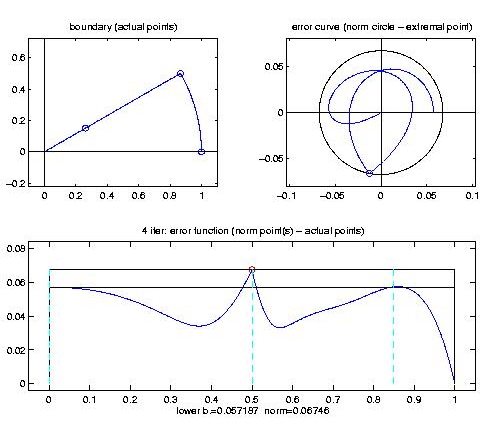
If you strike a key, the iteration starts and you will get extended output explaining the phases of the iteration. After improving the actual extremalpoint set, a figure occurs showing in position (2,2,1) the boundary of the region $\partial \Omega$ and the actual extremalpoint set (circles on the boundary). In position (2,2,2) you find a plot of the complex error function and in position (2,1,2) you find a plot of the absolute error function against the parametrisation interval [0,1]. A lower bound and upper bound for the error norm is shown and the candidates maximizing the error function are plotted.
- FUN =
name: 'fcos'
Showing you that the function is coded in the M-file fcos.m (c.f. directory approx). - BASIS =
name: 'monom' choice: [0 2 4 6] C_dim: 4
Showing you that the basis is coded in the M-file monom.m (c.f. directory basis). Additional parameter are specified: the complex dimension (in this case number of basis elements, C_dim=4) and particular choices of basis-function (in this case $\phi_j(z)=z^{j},\ j=0,2,4,6$ ). For details inspect monom.m. - BOUNDARY =
name: 'gcircle'
Showing you that the function is coded in the M-file gcircle.m (c.f. directory boundary). - Note:
You can always take the default parameters (see set_defaults.m)
However, if you like to modify some of them, this gives you an
idea how they look like.
PARA =
real_coef: 1 critical_points: [] initial_extremal_points: 'random' exchange: 'single' stepsize: 50 relative_error_bound: 1.0000e-03 iterations: 0 max_iterations: 15 initial_clustering: 0.0100 clustering_tolerance: 1.0000e-03 newton_tolerance: 1.0000e-10 newton_stepsize: 1.0000e-05 newton_iterations: 0 newton_max_iterations: 0 output: 'extended' plot: 'always: abserror+boundary' mywork: 'call cremez' oldwork: '' as_subroutine: 0 FUN: [1x1 struct] BASIS: [1x1 struct] BOUNDARY: [1x1 struct] C_dim: 4
Giving you information about the overall process. For details see set_default.m and set_para.m:- real_coef: flag, if 1, coefficients are assumed to be real numbers.
- critical_points: collects values t in ]0,1[ where the parametrisation is non-differentiable.
- initial_extremal_points: how to find initial extremal points.
- exchange: how to exchange extremal points.
- stepsize: number of discretisation points in [0,1], for finding discrete maximum of the error function.
- relative_error_bound: the relative error bound, stop iteration if (error_norm-lower_bound)/lower_bound <relative_error_bound.
- iterations: counter for performed iterations.
- max_iterations: maximum number of performed iterations.
- initial_clustering, clustering_tolerance: if (error_norm-lower_bound)/lower_bound < initial_clustering and $\vert t_j-t_k\vert\le$clustering_tolerance, extremal points properbly coincides. This motivates to terminate the complex remex algorithm (cremez.m) and start the (optional) second phase, a quasi Newton method (q_newton.m).
- newton_tolerance: stop the quasi Newton method if the norm of the gradient is less than newton_tolerance.
- newton_stepsize: for building the approximation to the hessian in the quasi Newton method.
- newton_iterations: counter for performed quasi Newton iterations.
- newton_max_iterations: maximum number of performed quasi Newton iterations (if newton_max_iterations=0, the second phase is disabled).
- output, plot: controls the amount of output (in the beginning you should use extended).
- mywork, oldwork: controls the outer loop of COCA, for details see coca.m.
- as_subroutine: enables you to run COCA as a subroutine (no menus).
- FUN, BASIS, BOUNDARY: collects your choices.
- C_dim: complex dimension of the approximation problem.
Fixed bugs
- 05-Dec-2001, basisfunction
[cheby.m]
now with derivatives (thanks to Pierre Montagnier from Acadia University, Wolfville, Canada) JM. - 13-Dec-2004, corrected a few typos (thanks to Alexis Humphreys) JM.

- People
- Johannes Bostelmann
- Daniel Budelmann
- Bernd Fischer
- Ole Gildemeister
- Stephanie Häger
- Stefan Heldmann
- Temke Kohlbrandt
- Annkristin Lange
- Jan Lellmann
- Tanja Loßau
- Johannes Lotz
- Jan Modersitzki
- Till Nicke
- Josephine Oettinger
- Nils Papenberg
- Sofie Saier
- Kerstin Sietas
- Angela Tesdorpf
- Herbert Thiele
- Johannes Voigts
- Sina Walluscheck
- Nick Weiss
- Sonja Wichelmann